오늘은 django진도 나가기로 했는데 전에 마저못했던것 복습했다ㅠㅠ
3. 멜론 100Chart_수집_분석_저장 이어서
iloc[row index, column index]
song_df.iloc[0:6, 0:4]
**mysql서버 켜기
mysql.server start
mysql -u python -p
show databases;
use python_db;
데이터프레임 객체를 DB에 저장하기
-
pymysql과 sqlalchemy 사용
pymysql : db와 연결
sqlalchemy : 객체를 테이블로 자동매핑
!pip install pymysqlCollecting pymysql
Downloading PyMySQL-1.0.2-py3-none-any.whl (43 kB)
|████████████████████████████████| 43 kB 327 kB/s eta 0:00:011
Installing collected packages: pymysql
Successfully installed pymysql-1.0.2
!pip show pymysqlName: PyMySQL
Version: 1.0.2
Summary: Pure Python MySQL Driver
Home-page: https://github.com/PyMySQL/PyMySQL/
Author: yutaka.matsubara
Author-email: yutaka.matsubara@gmail.com
License: "MIT"
Location: /Users/mhee4/opt/anaconda3/lib/python3.8/site-packages
Requires:
Required-by:
!pip show sqlalchemyName: SQLAlchemy
Version: 1.3.20
Summary: Database Abstraction Library
Home-page: http://www.sqlalchemy.org
Author: Mike Bayer
Author-email: mike_mp@zzzcomputing.com
License: MIT
Location: /Users/mhee4/opt/anaconda3/lib/python3.8/site-packages
Requires:
Required-by:
import pymysql
import sqlalchemy

# pymysql과 sqlalchemy 연동
pymysql.install_as_MySQLdb()
from sqlalchemy import create_engine

# engine 객체생성
engine = create_engine('mysql+mysqldb://python:python@localhost:3306/python_db', encoding='utf-8')
print(engine)

# engine을 사용해서 db에 연결
con = engine.connect()
print(con)

# DataFrame to_sql() 함수로 dataframe객체를 table로 저장
song_df.to_sql(name='songs', con=engine, if_exists='replace', index=False)
>>>Engine(mysql+mysqldb://python:***@localhost:3306/python_db)
<sqlalchemy.engine.base.Connection object at 0x7ff685376df0>
**terminal창에서
show tables;

desc songs;

select 곡명 from songs;

# dataframe을 excel file로 저장
song_df.to_excel('data/melon100차트.xlsx', sheet_name='멜론100')
sqlalchemy pandas
pymysql => db완성!
7.Pymysql과MariaDB연동(pymysql만으로 db연동하기)
sql = """
CREATE TABLE product (
    id INT UNSIGNED NOT NULL AUTO_INCREMENT,
    name VARCHAR(20) NOT NULL,
    model_num VARCHAR(10) NOT NULL,
    model_type VARCHAR(10) NOT NULL,
    PRIMARY KEY(id)
);
"""

sql
'\nCREATE TABLE product (\n id INT UNSIGNED NOT NULL AUTO_INCREMENT,\n name VARCHAR(20) NOT NULL,\n model_num VARCHAR(10) NOT NULL,\n model_type VARCHAR(10) NOT NULL,\n PRIMARY KEY(id)\n);\n'
import pymysql

db = pymysql.connect(host='localhost', port=3306, db='python_db',user='python',passwd='python',charset='utf8')
cursor = db.cursor()
cursor.execute(sql)
db.commit()
**terminal창에서
show tables;
desc product;
cursor.execute('drop table product')
cursor.execute('show tables')
>>>1
db.close()
import pymysql

#db와 연결
db = pymysql.connect(host='localhost', port=3306, db='python_db',user='python',passwd='python',charset='utf8')

try:
    #cursor 생성하고 cursor가 open되어 있는 query문을 여러개 실행
    with db.cursor() as cursor:
        #table drop하는 query 실행
        # cursor.execute('drop table product')
        #product table 생성 query실행
        cursor.execute(sql)
        #db에 실제로 적용한다
        db.commit()

        for num in range(10,20):
            name = 'S20'+str(num)
            ins_sql = \
                'insert into product (name,model_num,model_type) values (%s, %s, %s)'
                cursor.execute(ins_sql,(name,'7700','Phone'))
                print(ins_sql)
                # ins_sql = "insert into product (name,model_num,model_type) \
                # values('"+name+"','7700','Phone')"
                # cursor.execute(ins_sql)

        db.commit()
        print(cursor.lastrowid)
    except Exception as exp:
        print(exp)
        # db에 적용하지 말고 취소처리해라
        db.rollback()
    finally:
        db.close()
insert into product (name,model_num,model_type) values (%s, %s, %s)
insert into product (name,model_num,model_type) values (%s, %s, %s)
insert into product (name,model_num,model_type) values (%s, %s, %s)
insert into product (name,model_num,model_type) values (%s, %s, %s)
insert into product (name,model_num,model_type) values (%s, %s, %s)
insert into product (name,model_num,model_type) values (%s, %s, %s)
insert into product (name,model_num,model_type) values (%s, %s, %s)
insert into product (name,model_num,model_type) values (%s, %s, %s)
insert into product (name,model_num,model_type) values (%s, %s, %s)
insert into product (name,model_num,model_type) values (%s, %s, %s)
10
***terminal창
show tables;
select * from product;

import pymysql

db = pymysql.connect(host='localhost', port=3306, db='python_db',\
    user='python',passwd='python',charset='utf8')

try:
    #select, update
    with db.cursor() as cursor:
        cursor.execute('select * from product where id=3')
        result = cursor.fetchone()
        print(type(result),result, result[1])

        upd_sql = \
            "update product set model_type='%s' \
            where name between 'S2010' and 'S2015'" % '핸드폰'
            cursor.execute(upd_sql)
            db.commit()
            #갱신된 row 갯수
            print(cursor.rowcount)

            cursor.execute('select * from product')
            result_list = cursor.fetchall()
            print(type(result_list))
            for row in result_list:
                print(row[0],row[1],row[2],row[3])

            # model_type별로 group by 하는 쿼리 실행
            cursor.execute('select model_type,count(*) from product group by model_type')
            for row in cursor.fetchall():
                print(row)

       finally:
           db.close()
>>><class 'tuple'> (3, 'S2012', '7700', '핸드폰') S2012
0
<class 'tuple'>
1 S2010 7700 핸드폰
2 S2011 7700 핸드폰
3 S2012 7700 핸드폰
4 S2013 7700 핸드폰
5 S2014 7700 핸드폰
6 S2015 7700 핸드폰
7 S2016 7700 Phone
8 S2017 7700 Phone
9 S2018 7700 Phone
10 S2019 7700 Phone
('Phone', 4)
('핸드폰', 6)
# delete 하고 select all
#name 컬럼의 값이 's2014' 와 's2015' 인 행을 삭제하세요 sql의 in 구문을 사용하세요

con = pymysql.connect(host='localhost', port=3306, db='python_db',\
    user='python',passwd='python',charset='utf8')

#print(type(con), con)

try:
    with con.cursor() as cursor:
        sql = "delete from product where name in (%s,%s)"
        cursor.execute(sql,('S2012','S2013'))
        con.commit()
        # 삭제된 건수 출력
        print(cursor.rowcount)

        sql = "select * from product order by id"
        cursor.execute(sql)
        for row in cursor.fetchall():
            print(row[0],row[1],row[2],row[3])

except Exception as ex:
    con.rollback()
    print(ex)
finally:
    con.close()
>>>2
1 S2010 7700 핸드폰
2 S2011 7700 핸드폰
5 S2014 7700 핸드폰
6 S2015 7700 핸드폰
7 S2016 7700 Phone
8 S2017 7700 Phone
9 S2018 7700 Phone
10 S2019 7700 Phone
4. 행정구역정보분석 시각화
시각화
- jupyter notebook에서 플롯팅 옵션 설정
- matplotlib, seaborn 라이브러리 import
- 한글폰트 설정
#notebook 에 Plot이 그려지게 하기 위한 설정
#이 설정을 하면 show() 함수를 호출하지 않아도 Plot이 그려진다.
%matplotlib inline
import matplotlib
import matplotlib.pyplot as plt
import matplotlib.font_manager as fm
import seaborn as sns
print('matplotlib ', matplotlib.__version__)
print('seaborn ', sns.__version__)matplotlib 3.3.2
seaborn 0.11.0
#윈도우용 한글폰트참고
font_path = 'c:/windows/fonts/malgun.ttf'
font_prop = fm.FontProperties(fname=font_path).get_name()
#matplotlib의 rc(run command) 함수를 사용해서 한글폰트 설정
matplotlib.rc('font', family=font_prop)
#맥북용 한글폰트참고
from matplotlib import rc

rc('font', family='AppleGothic')
plt.rcParams['axes.unicode_minus'] = False- Figure 와 Axes 객체를 생성
- Figure는 그림이 그려지는 도화지
- Axes 는 Plot 이 그려지는 공간
- Figure에 Axes를 하나만 생성할 수도 있고,
- Figure에 Axes를 여러개 생성해서 화면을 분할 할 수도 있음
- seaborn에서 제공하는 막대그래프를 그릴 수 있는 barplot() 함수 사용
- 서울특별시의 행정구역별로 인구수
- 서울특별시의 행정구역별로 면적
seoul_df = data.loc[data['광역시도'] == '서울특별시']

figure,(axes1, axes2) = plt.subplots(nrows=2, ncols=1)
print(figure)
print(axes1)
print(axes2)
figure.set_size_inches(18,12)
seoul_pop_df = seoul_df.sort_values(by='인구수', ascending=False)
sns.barplot(x='행정구역', y='인구수', data=seoul_pop_df, ax=axes1)
seoul_area_df = seoul_df.sort_values(by='면적', ascending=False)
sns.barplot(x='행정구역', y='면적', data=seoul_area_df, ax=axes2)
>>>Figure(432x288)
AxesSubplot(0.125,0.536818;0.775x0.343182)
AxesSubplot(0.125,0.125;0.775x0.343182)

seoul_df = data.loc[data['광역시도'] == ['서울특별시']

#Figure와 Axes 객체 2개 생성
figure,(axes1,axes2)=plt.subplots(nrows=2, ncols=1)
#figure size 조절
figure.set_size_inches(18,12)
print(figure)
print(axes1)
print(axes2)

#barplot() - x축에는 행정구역, y축에는 인구수
sns.barplot(x='행정구역', y='인구수', \
            data=seoul_df.sort_values(by='인구수',ascending=False), ax=axes1)
#barplot() - x축에는 행정구역, y축에는 면적
sns.barplot(x='행정구역', y='면적', \
            data=seoul_df.sort_values(by='면적',ascending=False), ax=axes2)
>>>Figure(1296x864)
AxesSubplot(0.125,0.536818;0.775x0.343182)
AxesSubplot(0.125,0.125;0.775x0.343182)

def show_barplot(sido_name):
    sido_df = data.loc[data['광역시도'] == sido_name]

    #Figure와 Axes 객체 2개 생성
    figure,(axes1,axes2)=plt.subplots(nrows=2, ncols=1)
    #figure size 조절
    figure.set_size_inches(18,12)

    #barplot() - x축에는 행정구역, y축에는 인구수
    pop_plot = sns.barplot(x='행정구역', y='인구수', \
                data=sido_df.sort_values(by='인구수',ascending=False), ax=axes1)
    #해당 plot에 타이틀을 설정
    pop_plot.set_title(f'{sido_name} 행정구역별 인구수')

    #barplot() - x축에는 행정구역, y축에는 면적
    area_plot = sns.barplot(x='행정구역', y='면적', \
                data=sido_df.sort_values(by='면적',ascending=False), ax=axes2)
    area_plot.set_title(f'{sido_name} 행정구역별 면적')
show_barplot('강원도')
### 전국의 광역시도별 인구수 시각화
#figure와 axes 생성 - figure에 1개의 axes를 작성
figure,axes1 = plt.subplots(nrows=1, ncols=1)
#figure size를 확대
figure.set_size_inches(18,12)
print(figure)
print(axes1)

#광역시도별 인구수
sns.barplot(x='광역시도', y='인구수', data=data.sort_values(by='인구수',ascending=False),\
            ax=axes1)
>>>Figure(1296x864)
AxesSubplot(0.125,0.125;0.775x0.755)

5. 국회의원현황_스크래핑_분석_시각화_저장
->jupyter notebook 참고
-
Server-Side Rendering
-
: JSP, Thymeleaf, PHP, Django
-
: server에서 html작성해서 클라이언트로 내려주는 방식
-
: Synchronous(동기)방식으로 통신
-
->request(요청)을 보내고 응답(response)이 올때까지 클라이언트는 waiting 하는 방식
-
단점 : 화면 전체가 update 되어서 느림
-
Client-Side Rendering
-
: server에서는 data(xml, json, csv)를 내려주고, 클라이언트에서 html을 동적으로 작성하는 방식
-
: Ajax(Asynchronous Javascript and XML)
-
: Asynchronous(비동기) 방식으로 통신
-
-> request(요청)을 보내고 응답(response)을 waiting하지 않고, 다른 일을 하는 방식
-
-> javascript의 XmlHttpRequest(XHR)가 비동기 방식으로 통신을 해주는 역할을 담당한다.
**zip함수를 이용하여 list만들기
# zip 함수
dt_list = ['정당', '선거구']
dd_list = ['민주당', '서울은평구']
print(zip(dt_list,dd_list))
print(list(zip(dt_list,dd_list)))

for data in zip(dt_list, dd_list):
    print(type(data), data)

print(dict(zip(dt_list, dd_list)))
<zip object at 0x7f950909a740>
[('정당', '민주당'), ('선거구', '서울은평구')]
<class 'tuple'> ('정당', '민주당')
<class 'tuple'> ('선거구', '서울은평구')
{'정당': '민주당', '선거구': '서울은평구'}
**만 나이 구하기
from datetime import date

# 현재날짜
today = date.today()
print(today)
print(today.year)
print(today.month)
print(today.day)
2021-01-11
2021
1
11
# 1960 1 4
# 1960 12 5
birth = date(1960, 1, 4)
print(type(birth), birth)
print(birth.year)
print(birth.month)
print(birth.day)

birth2 = date(1960, 12, 5)
print(type(birth2), birth2)
print(birth2.year)
print(birth2.month)
print(birth2.day)
<class 'datetime.date'> 1960-01-04
1960
1
4
<class 'datetime.date'> 1960-12-05
1960
12
5
# 1-11 < 1-4(
today.month, today.day) < (birth.month, birth.day) # 0
False
(today.month, today.day) < (birth2.month, birth2.day) # 1True
# 1960 1 4
age1 = today.year - birth.year - ((today.month, today.day) < (birth.month, birth.day))
print(age1)
61
# 1960 12 5
age2 = today.year - birth2.year - ((today.month, today.day) < (birth2.month, birth2.day))
print(age2)
60
시각화
- 이미지 출력 - IPython에서 제공하는 Image 객체, display() 함수 사용
- seaborn - count plot(막대그래프), distplot(히스토그램,분포도)
- matplotlib - histogram, pie chart
- 한글폰트 설정
from IPython.display import Image, display

for image_url in member_df['이미지'].sample(3):
    print(image_url)
    # display(Image(url=image_url))
https://www.assembly.go.kr/photo/9770995.jpg
https://www.assembly.go.kr/photo/9771206.jpg
https://www.assembly.go.kr/photo/9770676.jpg
%matplotlib inline

import matplotlib
import matplotlib.pyplot as plt
import matplotlib.font_manager as fm
import seaborn as sns
#윈도우용 한글폰트참고
font_path = 'c:/windows/fonts/malgun.ttf'
font_prop = fm.FontProperties(fname=font_path).get_name()
#matplotlib의 rc(run command) 함수를 사용해서 한글폰트 설정
matplotlib.rc('font', family=font_prop)
#맥북용 한글폰트참고
from matplotlib import rc

rc('font', family='AppleGothic')
plt.rcParams['axes.unicode_minus'] = False
seaborn의 막대그래프
- barplot - x축, y축을 둘 다 설정할 수 있음
- countplot - x축 이나 y축 중에서 하나만 설정할 수 있음
member_df['정당'].value_counts()
member_df['정당'].value_counts().index

#figure와 axes 객체 생성
figure,(axes1,axes2) = plt.subplots(nrows=2, ncols=1)
figure.set_size_inches(18,12)

#정당과 당선횟수2 컬럼을 row count 것을 시각화
sns.countplot(data=member_df, x='정당', ax=axes1, order=member_df['정당'].value_counts().index)
sns.countplot(data=member_df, x='당선횟수2', ax=axes2, \
            order=member_df['당선횟수2'].value_counts().index)
#선거구2 컬럼의 값을 countplot으로 그리기
#figure에 axes 객체를 1개로 설정

figure, axes1 = plt.subplots(nrows=1, ncols=1)
figure.set_size_inches(18,12)
sns.countplot(data=member_df, y='선거구2', ax=axes1, \
            order=member_df['선거구2'].value_counts().index)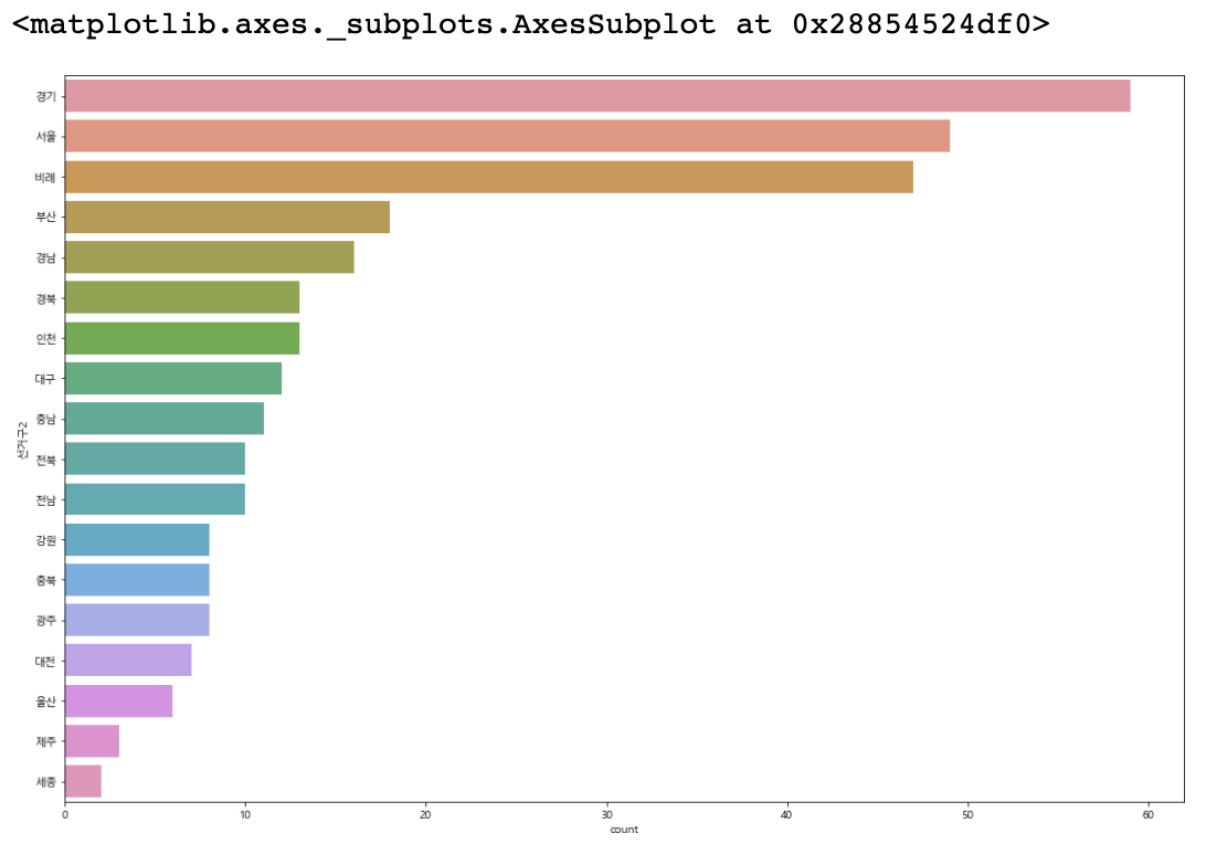
#산점도 seaborn의 scatterplot 를 사용
#선거구2 와 나이 분포도 를 확인
figure, (axes1,axes2) = plt.subplots(nrows=2, ncols=1)
figure.set_size_inches(18,12)
sns.scatterplot(data=member_df, x='선거구2', y='나이', ax=axes1)
sns.scatterplot(data=member_df, x='정당', y='나이', ax=axes2)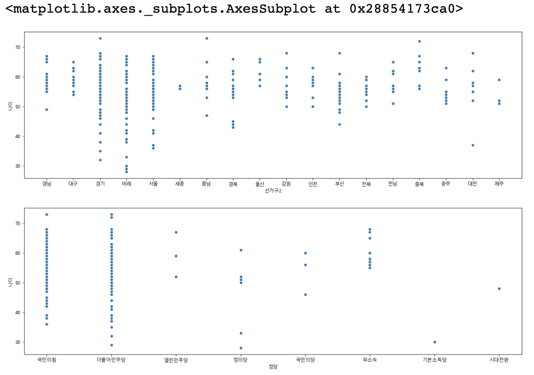
# 나이 값의 분포를 볼 수 있는 히스토그램 그릭
# seaborn의 distplot() 함수 사용
figure, axes1 = plt.subplots(nrows=1, ncols=1)
figure.set_size_inches(18,12)
sns.distplot(member_df['나이'], hist=True, ax=axes1)
#sns.distplot(member_df['나이'], hist=True)
age_df = member_df.loc[(member_df['나이'] > 35) & (member_df['나이'] < 65)]
len(age_df)
figure, axes1 = plt.subplots(nrows=1, ncols=1)
figure.set_size_inches(18,12)
sns.distplot(age_df['나이'], hist=True, ax=axes1)
#sns.distplot(age_df['나이'], hist=True)
#Matplotlib 를 사용하여 Histogram 그리기
arrays, bins, patches = plt.hist(member_df['나이'], bins=10)
print(arrays)
print(bins)
print(patches)
# row count를 퍼센티지(%) 비율로 나타내려면 value_counts(normalize=True) 로 설정
cdf = member_df['선거구2'].value_counts(normalize=True)
print(cdf.index)
cdf
Index(['경기', '서울', '비례', '부산', '경남', '경북', '인천', '대구', '충남', '전북', '전남', '강원', '충북', '광주', '대전', '울산', '제주', '세종'], dtype='object')
경기 0.196667 서울 0.163333 비례 0.156667 부산 0.060000 경남 0.053333 경북 0.043333 인천 0.043333 대구 0.040000 충남 0.036667 전북 0.033333 전남 0.033333 강원 0.026667 충북 0.026667 광주 0.026667 대전 0.023333 울산 0.020000 제주 0.010000 세종 0.006667 Name: 선거구2, dtype: float64
#Matplotlib의 pie plot 그리기

#figure size 조정
figure = plt.figure(figsize=(20,12))
#autopct는 값의 퍼센티지 포맷지정
#startangle은 첫번째 pie의 시작각도 지정
plt.pie(cdf, labels=cdf.index, autopct='%1.1f%%', startangle=140, shadow=True)
#pie plot을 그릴때 원의 형태를 유지하도록 하는 설정
plt.axis('equal')
plt.title('선거구 분포값')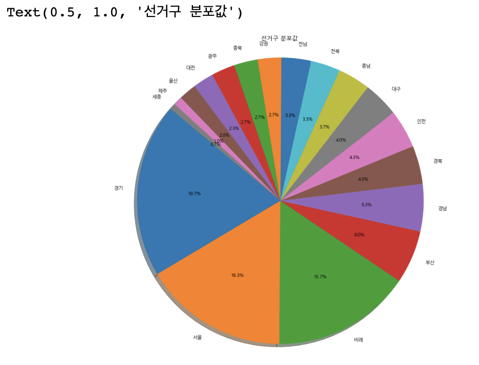
#pivot_table 함수 사용
age_pivot_df=member_df.pivot_table(index='나이',columns='정당',aggfunc='size').fillna(0).astype(int)
#.fillna(0).astype(int)
age_pivot_df.head()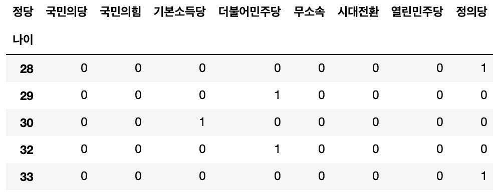
#seaborn의 heatmap 그리기
sns.heatmap(age_pivot_df, linewidths=1, annot=True, fmt='d')
#나이구간 컬럼을 추가
#print(member_df['나이'].value_counts())
member_df.loc[member_df['나이'] < 30,'나이구간'] = 20
member_df.loc[(member_df['나이'] >= 30) & (member_df['나이'] < 40),'나이구간'] = 30
member_df.loc[(member_df['나이'] >= 40) & (member_df['나이'] < 50),'나이구간'] = 40
member_df.loc[(member_df['나이']  >= 50) & (member_df['나이'] < 60),'나이구간'] = 50
member_df.loc[(member_df['나이'] >= 60) & (member_df['나이'] < 70),'나이구간'] = 60
member_df.loc[member_df['나이'] >= 70,'나이구간'] = 70

member_df['나이구간'].value_counts()
50 169 60 80 40 35 30 11 70 3 20 2
Name: 나이구간, dtype: int64
# 나이구간 컬럼의 타입을 변경 float -> int
member_df = member_df.astype({"나이구간":int})
member_df['나이구간'].dtype
dtype('int32')
age_pivot_df=member_df.pivot_table(index='나이구간',columns='정당',aggfunc='size')\
.fillna(0).astype(int)
age_pivot_df
sns.heatmap(age_pivot_df, linewidths=1, annot=True, fmt='d')
member_df.pivot_table(index='나이구간',columns='선거구2',aggfunc='size')
member_df.pivot_table(index='선거구2',columns='나이구간',aggfunc='size')
age_pivot_df2 = member_df.pivot_table(index='선거구3',columns='나이구간',aggfunc='size').fillna(0).astype(int)
age_pivot_df2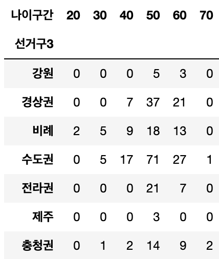
sns.heatmap(age_pivot_df2, annot=True, fmt='d', cmap=sns.light_palette('red'),\
            linewidths=0.5)
sns.heatmap(age_pivot_df2, annot=True, fmt='d',linewidths=0.5)
'CLOUD > Python' 카테고리의 다른 글
| 1/19 웹크롤링 - selenium, scrapy, 여러페이지 크롤링 (2) | 2021.01.19 |
|---|---|
| 1/18 웹스크래핑 - 복습, scrapy (0) | 2021.01.18 |
| 1/6 파이썬 5차시 - 웹스크래핑(csv, xml, json타입 처리), 데이터 분석 (0) | 2021.01.06 |
| 1/5 파이썬 4차시 - 깃파이참연동, 모듈과 패키지, 예외처리, 파일다루기, 웹스크래핑 (0) | 2021.01.05 |
| 1/4 파이썬 3차시 - 함수가이드라인, pythonic code, 람다, 객체와클래스, 모듈과 패키지 (0) | 2021.01.04 |